Re-examination · October 2026
Does a Hybrid Prophet-LSTM Forecast Stock Prices? A 2026 Re-examination of My MSc Thesis
Kaihuan Huang
Abstract
My 2024 MSc thesis proposed a hybrid of Prophet and a Long Short-Term Memory network (LSTM) for daily stock-price forecasting and reported that it was the best of four models on Apple, with a significant difference (p < 0.05). Two years later I reproduced the original code unchanged and evaluated it against the baseline it never used: the random walk, which forecasts that tomorrow's price equals today's. The random walk had the lowest error on all four series; the best thesis model was 1.9–5.6 times worse and the proposed hybrid 7.0–12.8 times worse (RMSE). I list twelve problems in the original study and measure each, including a 60-day misalignment in the hybrid, a scaler fitted on test data, and a reported test that does not exist in the code. I then re-ran the question under a current protocol: 20 US stocks and ETFs, log returns at 1, 5 and 20 trading days, a forecast from each of 208 trading days between November 2025 and September 2026 using only earlier data, and 16 models including the 2025 time-series foundation models Chronos-2 and TimesFM 2.5, each compared with the random walk by a Diebold-Mariano test. No model was significantly more accurate than the random walk at any horizon; the foundation models were significantly less accurate at one day, though their 80% intervals were close to calibrated. The result held on a second test period (2023–2025). The predictable quantity was volatility: a gradient-boosted model reduced the error of 20-day volatility forecasts by 20% against a naive baseline (relative MAE 0.802, DM p = 0.048, uncorrected for two comparisons). I close with what went wrong in how I worked, not only in the code, and the checklist I now apply before trusting any model result, including the language-model systems I build.
中文摘要 · 正文为英文
2024 年的硕士论文提出用 Prophet + LSTM 混合模型预测日股价,结论是它在苹果股票上最好,且差异显著(p < 0.05)。2026 年我用原代码原样复现,并加上论文从没用过的基准——随机游走(「明天的价格 = 今天的价格」):它在 4 个序列上误差都最小,论文最好的模型差 1.9–5.6 倍,混合模型差 7.0–12.8 倍。我列出原研究的 12 个问题并逐条量化,包括混合模型的 60 天错位、缩放器在测试数据上拟合、论文报告的检验在代码里不存在。随后按现在的协议重做:20 只美股和 ETF、1 / 5 / 20 天对数收益率、2025-11 到 2026-09 每个交易日一个预测起点(共 208 个,只用之前的数据)、16 个模型(含 2025 年的 Chronos-2、TimesFM 2.5),每个都用 Diebold-Mariano 检验和随机游走比较。没有任何模型在任何步长上显著优于随机游走;基础模型在 1 天上显著更差,但 80% 区间接近校准。换 2023–2025 测试期结论不变。能预测的是波动率:梯度提升树把 20 天波动率的预测误差降低 20%(相对 MAE 0.802,DM p = 0.048,未做两次比较的校正)。最后一节写我在做事方式上错在哪里(不只是代码),以及我现在相信任何模型结果之前都会过一遍的清单,包括我现在做的语言模型系统。
1Introduction
Forecasting daily stock prices is a standard student project because the data is free and the target feels important. It is also a setting where a weak evaluation can make almost any model look good: prices are highly autocorrelated, so any forecast close to yesterday's price earns a high R², and an error measured in dollars says nothing until it is compared with a sensible baseline.
This paper revisits my own MSc thesis with that in mind. It makes five contributions:
- An unchanged reproduction of the original code, matched to the result files submitted with the thesis (Section 3).
- A list of twelve problems in the original study, each with its measured effect (Section 4).
- A re-run of the research question under a 2026 protocol, with 16 models, two test periods and significance tests against the random walk (Sections 5–6).
- Evidence that, on the same data, volatility is predictable where direction is not (Section 6.4).
- An account of why the mistakes happened and the working checklist that came out of it (Section 8).
2The original study
- Data. Daily closing prices from yfinance, 1 January 2010 to 12 October 2024 (Google to 1 January 2023): Apple as the "stable" stock, Tesla as the "volatile" one, plus Google and the S&P 500.
- Split. One chronological split: the first 80% for training, the last 20% for testing (about October 2021 to October 2024; 655–744 trading days).
- Models. ARIMA(5,1,0); a two-layer LSTM with 50 units, a 60-day input window and MinMax-scaled prices, trained for 5 epochs; Prophet with yearly and weekly seasonality; and the hybrid, in which an LSTM predicts Prophet's residuals and the prediction is added back to Prophet's forecast.
- Metrics. MSE, RMSE, MAE, MAPE and R², computed on price levels.
- Claim. The hybrid is best on the stable stock, significantly so against the LSTM (p < 0.05), and worse than the LSTM on the volatile stock.
3Reproduction (E0)
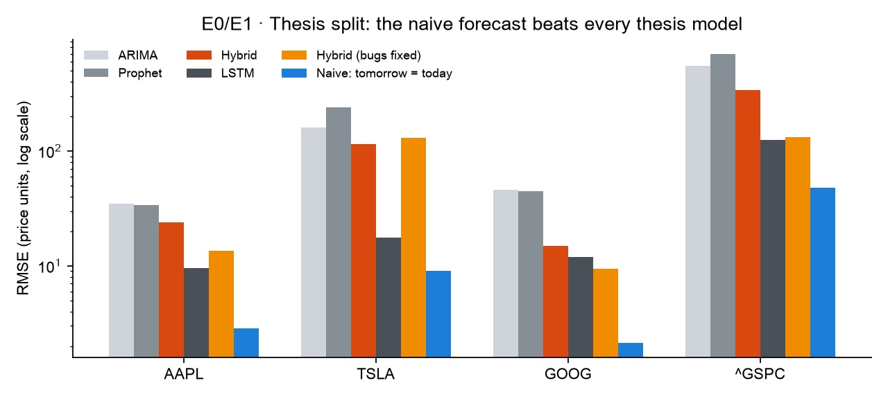
I ran the original functions without changing a line, with the same tickers, dates and split, over three random seeds. The results match the CSV files submitted with the thesis: the ARIMA RMSE for Tesla and the S&P 500 is identical (160.56 and 554.37), and Apple differs by 3% because today's download is dividend-adjusted. The problems below therefore belong to the study, not to the reproduction.
| Series | ARIMA | Prophet | LSTM | Hybrid | Random walk |
|---|---|---|---|---|---|
| AAPL | 34.8 | 33.9 | 9.5 | 24.0 | 2.85 |
| TSLA | 160.6 | 239.2 | 17.5 | 114.9 | 9.01 |
| GOOG | 45.9 | 44.9 | 11.9 | 14.9 | 2.14 |
| S&P 500 | 554.4 | 702.4 | 125.5 | 341.0 | 47.78 |
4Diagnosis: twelve problems (E1)
Listing 1 is the core of the hybrid as submitted. It contains two of the problems.
hybrid_prophet_lstm_forecast in the submitted app.py (abridged; line 4 summarises the training code).1residuals_full = total_dataset - prophet_full['yhat'].values
2scaler = MinMaxScaler(feature_range=(0, 1))
3residuals_scaled = scaler.fit_transform(residuals_full.reshape(-1, 1)) # fitted on train + test
4# ... train the LSTM on residual windows ...
5for i in range(len(train), len(total_dataset) - look_back):
6 X_test.append(residuals_scaled[i - look_back:i, 0])
7lstm_residuals = scaler.inverse_transform(lstm_model.predict(X_test))
8prophet_predictions_adjusted = prophet_predictions[look_back:] # shifted 60 days
9hybrid_predictions = prophet_predictions_adjusted + lstm_residuals.flatten()- No random-walk baseline. The random walk scores R² 0.97–0.99 on every series; the LSTM's R² of 0.84–0.95 only looked strong because prices are autocorrelated. The best thesis model's RMSE is 1.9–5.6 times the random walk's.
- The LSTM learned to copy yesterday, imprecisely. Its forecasts correlate 0.970–0.986 with the previous day's price, it calls the direction correctly 47.4–49.9% of the time, and with 5 epochs it is undertrained, so its error is about three times that of copying yesterday exactly.
- Unequal horizons. ARIMA and Prophet forecast 655–744 days ahead from the end of training; the LSTM and the hybrid forecast one day ahead with yesterday's true price as input. "LSTM beats ARIMA" reflects the protocol, not the models.
- A 60-day misalignment in the hybrid (Listing 1, line 8). The residual predicted for test day k is added to Prophet's forecast for day k + 60. Fixing only this reduces the hybrid's RMSE from 24.0 to 12.6 on Apple, 14.9 to 4.8 on Google and 114.9 to 66.6 on Tesla. Much of the thesis's "hybrid struggles in volatile markets" finding is this bug.
- Leakage (line 3). The scaler is fitted on training and test residuals together, so the model knows the test range. Fitting it on training data only raises the error on three of four series (Tesla 66.6 → 130.3, Google 4.8 → 9.4, Apple 12.6 → 13.5) and lowers it on the S&P 500 (153.2 → 131.8).
- Different test samples. The hybrid is scored on the test period minus its first 60 days; the other models on all of it.
- MinMax scaling of price levels cannot extrapolate. The training maximum maps to 1, so the LSTM cannot forecast a new high. On the 2025–2026 test period this setting is the worst of all models, 11.8 times the random walk's error.
- The conclusion contradicts the submitted results. The thesis names the hybrid best on Apple; the submitted
APPL_predict_results.csvreports RMSE 8.8 for the LSTM and 25.7 for the hybrid, with the hybrid's R² at −0.06. - Methods described but not implemented. The submitted code has no t-test behind the reported p < 0.05, no volume, moving-average or volatility features despite the described feature selection, no interpolation and no dropout tuning. K-fold appears only in an earlier version, and is not valid for time series.
- Metrics. MSE is not comparable across series (the S&P 500's is hundreds of times Apple's), R² on price levels is uninformative, and MAPE inflates errors on low-priced stocks.
- Sample. Two main stocks, one split, one training run: no estimate of variance.
- Engineering. Virtual environments,
node_modulesand a 1.4 GB archive were committed; versions were not pinned andrequirements.txtomitted TensorFlow and statsmodels.
5A 2026 protocol (E2)
- Data. 20 US stocks and ETFs (AAPL, TSLA, GOOG, MSFT, AMZN, NVDA, JPM, XOM, JNJ, PG, KO, WMT, CAT, BA, NFLX, AMD, PFE, DIS, SPY, QQQ), daily OHLCV adjusted for splits and dividends, January 2010 to September 2026, with SPY, VIX and the 10-year Treasury yield as exogenous series. Adjustment matters: Apple's 4-for-1 split in August 2020 would otherwise appear as a one-day log return of ln(1/4) ≈ −1.39.
- Target. The log return over the next h trading days, h ∈ {1, 5, 20}.
- Test period. 3 November 2025 to 1 September 2026, with a forecast origin on every trading day: 208 origins × 20 tickers = 4,160 forecasts per horizon. The period begins after the foundation models were released, so it cannot appear in their pre-training data.
- Training. Statistical models use only data up to each origin (ARIMA and ETS re-estimated every 20 origins and updated daily; Prophet refitted at every origin, 4,160 fits). Neural networks and gradient-boosted trees are trained once on data before 31 October 2025 and frozen; no target crosses into the test period.
- Models (16, scored against the random walk). Random walk with drift; AutoARIMA and AutoETS (statsforecast); the thesis family: Prophet, the price-level LSTM (thesis setting, leak removed), a return LSTM trained on the panel, and the hybrid with the misalignment fixed; PatchTST and NHITS (NeuralForecast); gradient-boosted trees on four data versions (Section 6.3); and zero-shot foundation models Chronos-Bolt-base (released November 2024), Chronos-2 (October 2025) and TimesFM 2.5 (September 2025).
- Metrics and tests. MAE relative to the random walk (below 1 beats it), out-of-sample R² against the random walk, directional accuracy compared with always predicting a rise, 80% interval coverage, pinball loss, and at h = 1 the annualised Sharpe ratio of a long-short rule after 2 basis points of cost. Each model is compared with the random walk by a Diebold-Mariano test on the cross-sectional mean loss differential, with a Newey-West variance at lag h − 1 and the Harvey-Leybourne-Newbold small-sample correction.
6Results
6.1 Main test period, November 2025 – September 2026
| Model | Rel. MAE | R²oos | Direction | p | 80% cover | Sharpe |
|---|---|---|---|---|---|---|
| Random walk with drift | 1.000 | 0.00% | 51.2% | 0.98 | 82.7% | 0.81 |
| GBDT, panel + technical | 1.001 | 0.05% | 51.3% | 0.88 | 75.8% | 1.44 |
| AutoETS | 1.002 | −0.17% | 49.8% | 0.45 | 83.2% | 0.58 |
| AutoARIMA | 1.007 | −1.12% | 48.6% | 0.006 | 81.0% | −2.18 |
| Return LSTM (3 seeds) | 1.010 | −0.99% | 50.2% | 0.40 | – | 0.60 |
| PatchTST | 1.012 | −2.26% | 50.0% | 0.002 | – | −0.89 |
| TimesFM 2.5 | 1.019 | −2.40% | 49.7% | 0.001 | 84.6% | −0.70 |
| Chronos-2 | 1.059 | −9.46% | 50.6% | <0.001 | 79.4% | −1.25 |
| NHITS | 1.059 | −9.81% | 49.6% | <0.001 | – | −0.75 |
| Chronos-Bolt-base | 1.140 | −22.9% | 51.0% | <0.001 | 80.0% | −1.20 |
| Hybrid Prophet-LSTM (fixed) | 1.220 | −55% | 49.5% | <0.001 | – | −0.95 |
| Prophet | 3.468 | −1053% | 50.4% | <0.001 | 57.2% | −0.29 |
| Price-level LSTM (thesis) | 11.758 | −11432% | 48.4% | <0.001 | – | −0.76 |
| Always up / buy and hold | 51.3% | 1.18 |
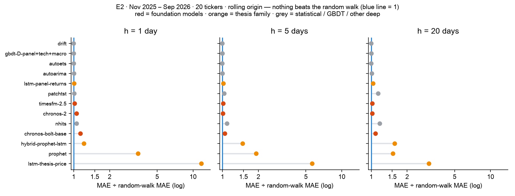
No model is significantly more accurate than the random walk. The best (random walk with drift, gradient-boosted trees, AutoETS) tie it at relative MAE 1.000–1.002; every model with p < 0.05 is significantly worse. The ranking at 5 and 20 days is similar: the best models sit at 0.998–1.008 with p above 0.6, the foundation models at 1.011–1.088, and both Chronos models are significantly worse than the random walk at the 5% level. At 20 days the gradient-boosted models call the direction correctly 54.1–54.5% of the time, the same as always predicting a rise (54.4%).
The foundation models' median forecasts move by 0.4–0.7% a day, but those moves are essentially uncorrelated with what happened (−0.16 for Chronos-Bolt at 20 days), so they add noise to a near-zero signal. Their strength is uncertainty: TimesFM 2.5's 80% intervals cover 84.6% of outcomes and Chronos-Bolt's 80.0%. The Sharpe ratios are not distinguishable: with 208 days (0.83 years) their standard error is roughly ±1.1–1.4, so 1.44 for gradient-boosted trees and 1.18 for buy-and-hold are within noise. Prophet, which has no autoregressive term, forecasts a return to its trend line every day; the price-level LSTM cannot forecast above its training maximum.
6.2 Robustness: January 2023 – October 2025 (E3)
I re-ran the less expensive models on an earlier period: 711 origins × 20 tickers = 14,220 forecasts per horizon, training ending 30 December 2022. This period may overlap the foundation models' pre-training data, which can only favour them.
| Model | h=1 | p | h=5 | p | h=20 | p | Direction, h=20 |
|---|---|---|---|---|---|---|---|
| Random walk with drift | 0.997 | 0.13 | 0.990 | 0.12 | 0.971 | 0.13 | 60.5% |
| GBDT A, one ticker, own lags | 0.998 | 0.25 | 0.989 | 0.10 | 0.965 | 0.08 | 60.4% |
| GBDT C, panel + technical | 1.000 | 0.60 | 0.989 | 0.14 | 0.976 | 0.19 | 59.4% |
| GBDT D, + macro | 1.004 | 0.89 | 0.993 | 0.48 | 0.970 | 0.12 | 59.1% |
| AutoETS | 0.999 | 0.47 | 0.992 | 0.04 | 0.974 | 0.07 | 58.2% |
| AutoARIMA | 1.002 | 0.77 | 0.993 | 0.19 | 0.974 | 0.20 | 59.5% |
| TimesFM 2.5 | 1.019 | <0.001 | 1.007 | 0.14 | 1.002 | 0.67 | 54.1% |
| Chronos-2 | 1.055 | <0.001 | 1.013 | 0.02 | 1.003 | 0.11 | 55.2% |
| Chronos-Bolt-base | 1.157 | <0.001 | 1.053 | <0.001 | 1.050 | 0.02 | 54.1% |
| Always up | 60.4% |
This was a strong bull market (equal-weight buy-and-hold Sharpe 1.63), so drift alone improves on the random walk by 3% at 20 days. The learned models improve by the same amount, and their 60.4% directional accuracy equals always predicting a rise: they learned that prices tend to go up, and nothing more. The only p < 0.05 in favour of a model is AutoETS at five days (p = 0.04), one result among 30 model-horizon pairs, which does not survive a multiple-comparison correction. The foundation models rank last again.
6.3 What better data buys (E4)
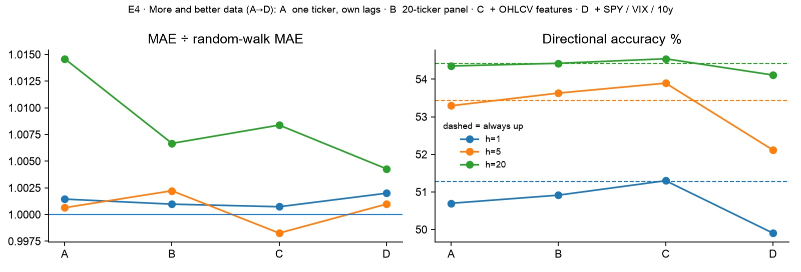
Holding the learner fixed (gradient-boosted trees with quantile loss), I varied only the data: (A) one model per ticker on its own lagged returns, the thesis's information set; (B) one model on the 20-ticker panel; (C) B plus OHLCV features (5-, 20- and 60-day returns and volatility, distance from moving averages, volume z-score, intraday range); (D) C plus market and macro series (lagged SPY return, VIX level and change, 10-year yield change).
| Version | Rel. MAE h=1 | h=5 | h=20 | 80% cover, h=1 | Rel. pinball, h=1 |
|---|---|---|---|---|---|
| A one ticker, own lags | 1.001 | 1.001 | 1.015 | 74.3% | 0.999 |
| B panel | 1.001 | 1.002 | 1.007 | 76.8% | 0.999 |
| C + technical | 1.001 | 0.998 | 1.008 | 75.8% | 0.992 |
| D + macro | 1.002 | 1.001 | 1.004 | 75.2% | 0.993 |
More and better data barely moves point accuracy: at most 1% (20 days, A to D), and nothing is significant. The gain is in the intervals: volatility features lower pinball loss by about 0.8%, because volatility is predictable (Section 6.4). The larger gain from data work is avoiding mistakes: adjusted prices, returns rather than levels, features dated no later than the origin, and targets that never cross into the test period together bring the thesis family from 3–12 times the random walk's error back to about 1.0 (return LSTM 1.010).
6.4 Volatility is predictable (E5)
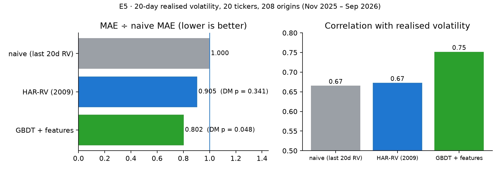
With the same tickers and origins, I changed the target to realised volatility over the next 20 days.
| Model | Rel. MAE | R²oos vs naive | QLIKE | Correlation | p |
|---|---|---|---|---|---|
| Naive (last 20 days) | 1.000 | 0% | 0.283 | 0.665 | – |
| HAR-RV (Corsi, 2009) | 0.905 | +15.2% | 0.261 | 0.673 | 0.34 |
| GBDT, version D features | 0.802 | +32.8% | 0.207 | 0.752 | 0.048 |
Gradient-boosted trees reduce the error of 20-day volatility forecasts by 20% (relative MAE 0.802, out-of-sample R² +32.8%). The effect is large but the evidence is only marginally significant (DM p = 0.048), for a clear reason: adjacent 20-day windows overlap by 19 days, so each ticker contributes roughly 208 ÷ 20 ≈ 10 independent observations, and the 20 tickers move together when VIX moves. Two models were tested against the naive forecast; a Bonferroni correction gives 0.048 × 2 = 0.096, above 0.05. The defensible statement is the effect size with a qualified test, not a pass at 0.05. Direction is noise; volatility clusters.
7Discussion
Why nothing beats the random walk. The result is consistent with the efficient-markets view (Fama, 1970) and with the forecasting literature, where simple benchmarks are hard to beat out of sample (Welch & Goyal, 2008). A regularity that public models can find in public daily prices is one that traders can exploit, and exploiting it removes it. Tying the random walk is the realistic ceiling for this task.
What changed between 2024 and 2026. The tools changed a great deal: statsforecast and NeuralForecast run rolling-origin evaluation in a few lines, and a zero-shot foundation model produces 4,160 forecasts with intervals in seconds (Chronos-Bolt took 22 seconds on an M1 Pro). On general benchmarks such as GIFT-Eval these models now beat classical methods. On daily stock returns their point accuracy did not improve, and should not be expected to. What changed most is the standard of evaluation: the first question a reviewer asks today is whether the model was compared with the random walk.
What the thesis should have asked. A falsifiable version of the question is: can 2025 time-series foundation models, zero-shot, beat classical baselines on stock returns and volatility? Stated as hypotheses: H1, no model is significantly more accurate than the random walk on returns (supported); H2, learned models beat naive and HAR forecasts of volatility (partly supported: GBDT at p = 0.048, HAR not significant); H3, foundation-model intervals are better calibrated than a Gaussian random walk (not tested here).
8Reflection: what I got wrong, and how I work now
The errors in Section 4 are symptoms. This section is about the habits that produced them, because those habits would produce the same errors on any other problem.
8.1 Why the mistakes happened
- Nothing had to be beaten. The study compared four models with each other and never with a forecast they had to beat. That produces a ranking, and a ranking always has a winner, so the study could not fail. The question I should have asked first was "what does doing nothing clever score?"
- I read a high number as success. An R² of 0.9 looked like a good model. I did not ask what a trivial forecast would score on the same metric; the answer, 0.99, would have ended the thesis's argument on the first day.
- The write-up drifted from the code. The methods chapter describes a t-test, feature selection and interpolation that are not in the submitted code, and the conclusion contradicts the submitted results file. I wrote what I had planned and believed, and did not check each sentence against an output.
- Nothing forced the predictions to line up. The 60-day shift survived because forecasts and targets were matched by array position, never by date, and no test checked that day k's forecast was compared with day k's price. The leak survived because preprocessing was fitted before the split rather than inside it.
- One run was treated as the answer. One split, one training run, no second period. With no variance, I could not tell a result from noise, and neither could a reader.
- I could not have re-run it myself. An unpinned environment and a repository full of build artefacts meant that even I could not reproduce the numbers later. A result nobody can re-run, including its author, cannot be corrected.
8.2 What I learned
- A model's score is a claim about a comparison. Without a baseline and a test, it is not yet a result.
- The evaluation is designed before the model, not after. The split, the baseline, the metric and the bar to clear decide what the study can conclude. Changing them after seeing results is how a study ends up proving what its author hoped.
- Bugs hide in summary tables. Neither bug was visible in the table of RMSEs. Both appeared only when I aligned forecasts to dates and refitted preprocessing on training data alone.
- An honest negative result is useful. Accepting that daily returns are not predictable is what led to the question that was answerable: volatility (Section 6.4).
- Better tools do not fix the question. The 2026 tools made the re-run fast and the foundation models are strong elsewhere, but none of them could beat the random walk on this target. Model capability is moving quickly; whether a result can be trusted still depends on the protocol.
8.3 How I work now
Before I trust any model result, mine or anyone else's, I go through this list:
- Baseline and bar first. Before building anything, write down the simplest baseline (the random walk, a rule, no model at all) and how much better the model must be to matter.
- Freeze the test set before looking. Split by time or by source. Nothing from the test set touches scaling, feature selection, prompts, few-shot examples or fine-tuning data.
- Join on keys, and assert it. Forecasts and targets are matched by date or ID, and the code fails if they do not line up.
- Same samples, same information. Every model sees the same rows, the same horizon and the same inputs, or the difference is stated next to the number.
- Effect size with uncertainty. Report how big the difference is, with a test, seeds or an interval, and correct for the number of comparisons.
- A second period or dataset before calling anything a finding.
- Every sentence traceable. Each claim in a write-up points to a file or a line of code, and tables are generated from result files rather than typed. The video's numbers are read directly from the result files; the tables on this page were transcribed from them, and generating them too is the next step.
- One-command re-run. Pinned environment, data snapshot, scripts in order.
- Ask whether the target is predictable at all, and change the question if it is not.
The same list applies to the language-model systems I build now. On the Booking Agent, the rules and the confirmation gate are measured on a separate held-out set of 39 cases, and the page says plainly that this and the 30-case pilot are not a like-for-like before-and-after. On the PII detector, recall is reported per category rather than as one average, which is how the Chinese national-ID gap (23% before boundary-safe rules, 91% after) became visible. Evaluating a prompt or an agent has the same traps as evaluating a forecaster: no baseline, test examples leaking into prompts, and a single run read as a result.
9Limitations
- Moirai 2 and TimesFM 3 were not run: Moirai 2's library pins PyTorch 2.4 and NumPy 1.x, which conflicted with the other packages, and TimesFM 3 is a separate package. Chronos-2 was run without covariates.
- LightGBM needed a system OpenMP library, so scikit-learn's HistGradientBoosting (the same family of algorithm) was used instead.
- The main test period is 11 months, which limits the power of the Sharpe comparison and the 20-day tests.
- No multiple-comparison correction was applied across 16 models and 3 horizons. No model was significantly better, so a correction would not change the conclusion.
- Only public daily data was used: no intraday data, news or order flow.
10Conclusion
The thesis's central claim does not survive reproduction: its models lose to the random walk by a wide margin, and part of what it reported came from a misalignment and a leak in the code. Under a current protocol, 16 models including 2025's foundation models do not significantly beat the random walk on daily stock returns, on two test periods. What is predictable on the same data is volatility. The broader lesson is that as models improve, the evaluation protocol, not the model, decides whether a result can be trusted. The habits behind the original errors, and the checklist I use now, are in Section 8.
Reproducibility
The original code and result files, the new experiment code, all forecasts and scores, and a locked environment (uv, requirements.lock.txt) are kept together; the full run takes about one hour on an M1 Pro with 16 GB of memory. The repository is not yet public. A narrated walkthrough of the study is on the case page.
References
- Ansari, A. F., et al. (2024). Chronos: Learning the language of time series. Transactions on Machine Learning Research.
- Aksu, T., et al. (2024). GIFT-Eval: A benchmark for general time series forecasting model evaluation. arXiv:2410.10393.
- Challu, C., et al. (2023). NHITS: Neural hierarchical interpolation for time series forecasting. AAAI 2023.
- Corsi, F. (2009). A simple approximate long-memory model of realized volatility. Journal of Financial Econometrics, 7(2), 174–196.
- Das, A., Kong, W., Sen, R., & Zhou, Y. (2024). A decoder-only foundation model for time-series forecasting. ICML 2024.
- Diebold, F. X., & Mariano, R. S. (1995). Comparing predictive accuracy. Journal of Business & Economic Statistics, 13(3), 253–263.
- Fama, E. F. (1970). Efficient capital markets: A review of theory and empirical work. Journal of Finance, 25(2), 383–417.
- Harvey, D., Leybourne, S., & Newbold, P. (1997). Testing the equality of prediction mean squared errors. International Journal of Forecasting, 13(2), 281–291.
- Hochreiter, S., & Schmidhuber, J. (1997). Long short-term memory. Neural Computation, 9(8), 1735–1780.
- Hyndman, R. J., & Khandakar, Y. (2008). Automatic time series forecasting: The forecast package for R. Journal of Statistical Software, 27(3).
- Newey, W. K., & West, K. D. (1987). A simple, positive semi-definite, heteroskedasticity and autocorrelation consistent covariance matrix. Econometrica, 55(3), 703–708.
- Nie, Y., Nguyen, N. H., Sinthong, P., & Kalagnanam, J. (2023). A time series is worth 64 words: Long-term forecasting with transformers. ICLR 2023.
- Taylor, S. J., & Letham, B. (2018). Forecasting at scale. The American Statistician, 72(1), 37–45.
- Welch, I., & Goyal, A. (2008). A comprehensive look at the empirical performance of equity premium prediction. Review of Financial Studies, 21(4), 1455–1508.